Static graphs are a big improvement over no graphs but we can all agree that static information is not particularly engaging. On the web there is no presenter to talk over a picture. It is the role of a visualisation to grab the reader’s attention and get its point across. Making a graph interactive is a good step towards increasing its understandability. This post in an addendum to the previous tutorial on how to make a line chart. It will explore two techniques of making the previous project interactive.
Document Setup
If you’d like to follow this tutorial, create the following files in your project folder: line_chart_interactive.html, data.csv, more_data.csv, and styles.css. The files are almost exact copies of the ones used in the line chart tutorial, with the exception of additional section placeholders and a new file, more_data.csv that carries additional data series.
This should go to line_chart_interactive.html:
<!DOCTYPE html>
<head>
<meta charset="utf-8">
<title>Multi Line Chart</title>
<script type="text/javascript" src="https://d3js.org/d3.v5.min.js"></script>
<link rel="stylesheet" type="text/css" href="styles.css">
<style></style>
</head>
<body>
<div id="container" class="svg-container"></div>
<script>
//------------------------1. PREPARATION------------------------//
//-----------------------------SVG------------------------------//
const width = 960;
const height = 500;
const margin = 5;
const padding = 5;
const adj = 30;
// we are appending SVG first
const svg = d3.select("div#container").append("svg")
    .attr("preserveAspectRatio", "xMinYMin meet")
    .attr("viewBox", "-"
          + adj + " -"
          + adj + " "
          + (width + adj *3) + " "
          + (height + adj*3))
    .style("padding", padding)
    .style("margin", margin)
    .classed("svg-content", true);

//-----------------------------DATA-----------------------------//
const timeConv = d3.timeParse("%d-%b-%Y");
const dataset = d3.csv("data.csv");
dataset.then(function(data) {
    var slices = data.columns.slice(1).map(function(id) {
        return {
            id: id,
            values: data.map(function(d){
                return {
                    date: timeConv(d.date),
                    measurement: +d[id]
                };
            })
        };
    });

//----------------------------SCALES----------------------------//
const xScale = d3.scaleTime().range([0,width]);
const yScale = d3.scaleLinear().rangeRound([height, 0]);

xScale.domain(d3.extent(data, function(d){
    return timeConv(d.date)}));

yScale.domain([(0), d3.max(slices, function(c) {
    return d3.max(c.values, function(d) {
        return d.measurement + 4; });
        })
    ]);

//-----------------------------AXES-----------------------------//
const yaxis = d3.axisLeft()
    .ticks((slices[0].values).length)
    .scale(yScale);

const xaxis = d3.axisBottom()
    .ticks(d3.timeDay.every(1))
    .tickFormat(d3.timeFormat('%b %d'))
    .scale(xScale);

//----------------------------LINES-----------------------------//
const line = d3.line()
    .x(function(d) { return xScale(d.date); })
    .y(function(d) { return yScale(d.measurement); });

let id = 0;
const ids = function () {
    return "line-"+id++;
}

//---------------------------TOOLTIP----------------------------//


//-------------------------2. DRAWING---------------------------//
//-----------------------------AXES-----------------------------//
svg.append("g")
    .attr("class", "axis")
    .attr("transform", "translate(0," + height + ")")
    .call(xaxis);

svg.append("g")
    .attr("class", "axis")
    .call(yaxis)
    .append("text")
    .attr("transform", "rotate(-90)")
    .attr("dy", ".75em")
    .attr("y", 6)
    .style("text-anchor", "end")
    .text("Frequency");

//----------------------------LINES-----------------------------//
const lines = svg.selectAll("lines")
    .data(slices)
    .enter()
    .append("g");

    lines.append("path")
    .attr("class", ids)
    .attr("d", function(d) { return line(d.values); });

    lines.append("text")
    .attr("class","serie_label")
    .datum(function(d) {
        return {
            id: d.id,
            value: d.values[d.values.length - 1]}; })
    .attr("transform", function(d) {
            return "translate(" + (xScale(d.value.date) + 10)
            + "," + (yScale(d.value.measurement) + 5 )+ ")"; })
    .attr("x", 5)
    .text(function(d) { return ("Serie ") + d.id; });

//---------------------------POINTS-----------------------------//

//---------------------------EVENTS-----------------------------//

});
</script>
</body>
This should go to styles.css:
/* AXES */
/* ticks */
.axis line{
stroke: #706f6f;
stroke-width: 0.5;
shape-rendering: crispEdges;
}

/* axis contour */
.axis path {
stroke: #706f6f;
stroke-width: 0.7;
shape-rendering: crispEdges;
}

/* axis text */
.axis text {
fill: #2b2929;
font-family: Georgia;
font-size: 120%;
}

/* LINE CHART */
path.line-0 {
fill: none;
stroke: #ed3700;
}

path.line-1 {
fill: none;
stroke: #2b2929;
stroke-dasharray: 2;
}

path.line-2 {
fill: none;
stroke: #9c9c9c;
stroke-dasharray: 6;
}

.serie_label {
fill: #2b2929;
font-family: Georgia;
font-size: 80%;
}
These are the contents of data.csv:
date,A,B,C
20-Jul-2019,10,20,16
21-Jul-2019,11,22,18
22-Jul-2019,13,19,21
23-Jul-2019,11,17,22
24-Jul-2019,15,16,20
25-Jul-2019,16,19,18
26-Jul-2019,19,21,18
27-Jul-2019,22,25,15
28-Jul-2019,18,24,12
29-Jul-2019,14,20,16
30-Jul-2019,14,18,18
31-Jul-2019,16,18,21
01-Aug-2019,15,20,22
02-Aug-2019,14,21,19
And finally, this is what more_data.csv should contain:
date,A,B,C,D,E,F,G,H,I,J
20-Jul-2019,10,20,16,8,19,18,12,9,10,15
21-Jul-2019,11,22,18,10,21,22,11,9,12,15
22-Jul-2019,13,19,21,11,22,20,8,10,12,17
23-Jul-2019,11,17,22,15,23,19,10,9,14,16
24-Jul-2019,15,16,20,12,24,22,11,13,15,16
25-Jul-2019,16,19,18,11,22,22,13,13,14,16
26-Jul-2019,19,21,18,10,25,23,14,14,16,14
27-Jul-2019,22,25,15,14,27,23,15,12,17,15
28-Jul-2019,18,24,12,14,25,20,14,10,18,16
29-Jul-2019,14,20,16,17,27,17,14,12,17,18
30-Jul-2019,14,18,18,14,28,17,14,8,19,17
31-Jul-2019,16,18,21,13,30,15,15,7,22,20
01-Aug-2019,15,20,22,12,28,16,13,7,20,19
02-Aug-2019,12,21,19,10,28,17,14,8,20,22
Once you save the files and refresh the browser, the following graph will be displayed on your screen:
Earlier this week we studied the importance of differentiating between data series. Each line on the graph is distinguished by its unique colour and stroke. The series are labeled; the label is placed right next to the data it represents to minimise the eye movement. This technique facilitates an immediate comparative analysis of the series for the graph consumer. Placing the label under the graph (as it is standard for MS Excel graphs, for example) or revealing it on a mouse-over tends to decrease its analytical quality.
Introducing interactive elements on a visualisation should only be done to enhance its readability. The following sections explore two scenarios in which dynamic elements add to the overall user experience.
Scenario 1: Focus on Details
The first scenario adds dynamic detail to the visualisation and reduces the cognitive effort required to correctly interpret the graph. Currently, to get the value of a particular data point, the viewer has to read it off the y axis, drawing an imaginary line from the point of interest to the axis. This minimal movement takes the viewer’s eyes off the centre of the graph and can potentially introduce an error in reading. To counteract this effect, we can display the value as soon as the viewer’s eyes (and the cursor) land on the point of interest.
Technically speaking, we will introduce mouse events to the visualisation. As soon as the cursor is over a data point, a tooltip with the data value will be displayed. As soon as the cursor moves from the data point, the tooltip disappears.
To do this, we have to define a tooltip, draw data points on the lines (at the moment it’s not clear which elements are responsive), create an invisible area to hover over (the area should be larger than the point itself to increase the interactive real estate), and define the event structure.
Paste the following to the TOOLTIP section:
const tooltip = d3.select("body").append("div")
    .attr("class", "tooltip")
    .style("opacity", 0)
    .style("position", "absolute");
The snippet defines a tooltip that will be displayed on a hover over a data point. It will only become visible then, so its default opacity is set to 0.
Append the tooltip’s aesthetics to styles.css:
/* TOOLTIP */
.tooltip {
fill: #2b2929;
font-family: Georgia;
font-size: 150%;
}
Once the tooltip is defined, let’s add points to the chart lines. Paste the following bit in the POINTS section of the html document:
lines.selectAll("points")
    .data(function(d) {return d.values})
    .enter()
    .append("circle")
    .attr("cx", function(d) { return xScale(d.date); })
    .attr("cy", function(d) { return yScale(d.measurement); })
    .attr("r", 1)
    .attr("class","point")
    .style("opacity", 1);
Define the points in styles.css:
/* POINTS */
.point {
stroke: none;
fill: #9c9c9c;
}
After the page is refreshed in the browser, the newly created data points become visible on the lines representing the data series:
Now let’s proceed to the core of this section: the mouse events. As the first step, we need to specify an element that can be hovered over. In theory it can be our current data points. I’d recommend against it: these points are so tiny that placing the cursor directly over them would become a sniper exercise on its own and might, in result, hamper the viewer’s attention. I suggest that we use invisible elements instead and increase the tooltip activation area. Since the points are shaped as circles, we could construct an invisible – but larger – circle around each of them. Hovering over that area will activate the tooltip and, in result, improve the overall interaction.
Paste the following to the EVENTS section:
lines.selectAll("circles")
    .data(function(d) { return(d.values); } )
    .enter()
    .append("circle")
    .attr("cx", function(d) { return xScale(d.date); })
    .attr("cy", function(d) { return yScale(d.measurement); })
    .attr('r', 10)
    .style("opacity", 0)
Note how the code is almost exactly the same as the earlier snippet that added the data points. The major differences here are the increased circle radius and the element’s opacity set to 0.
The next step is configuring the events. We need to specify what happens when the mouse is over a circle, and what is expected after the mouse moves from it. Append the following to the ghost circles definition:
// current code
    lines.selectAll("circles")
    .data(function(d) { return(d.values); })
    .enter()
    .append("circle")
    .attr("cx", function(d) { return xScale(d.date); })
    .attr("cy", function(d) { return yScale(d.measurement); })
    .attr('r', 10)
    .style("opacity", 0)

//append this
    .on('mouseover', function(d) {
        tooltip.transition()
            .delay(30)
            .duration(200)
            .style("opacity", 1);

        tooltip.html(d.measurement)
        .style("left", (d3.event.pageX + 25) + "px")
        .style("top", (d3.event.pageY) + "px")
    })

    .on("mouseout", function(d) {
        tooltip.transition()
        .duration(100)
        .style("opacity", 0);
    });
The syntax of the events is as follows:
.on([event], [do something])
We are working with two events in this example: mouse over an element, and mouse out. On the mouse over we want to display a tooltip, which is as simple as changing its opacity to 1. We also need to configure the text to display (the measurement associated with a point) and give the tooltip a position on the plane. Those coordinates are generated dynamically by reading the current position of the cursor. On mouse out we simply hide the tooltip away.
If you’d like to study the mouse events further there is a good read on selections in D3.js from D3 in Depth.
Save the html file and interact with the visualisation – the tooltip comes and goes as we get closer to or further from a data point!
The chart can be further improved by visually emphasizing the selected data point: it would serve as a confirmation for the viewer that they are looking at the right element. This can be done by increasing the circle radius on a hover. The invisible circles we use as hover areas will work great for this purpose. They just need to be made visible on a selection.
Add the following bits to the mouse on and mouse out events:
lines.selectAll("circles")
    .data(function(d) { return(d.values); } )
    .enter()
    .append("circle")
    .attr("cx", function(d) { return xScale(d.date); })
    .attr("cy", function(d) { return yScale(d.measurement); })
    .attr('r', 10)
    .style("opacity", 0)
    .on('mouseover', function(d) {
        tooltip.transition()
        .delay(30)
        .duration(200)
        .style("opacity", 1);

        tooltip.html(d.measurement)
            .style("left", (d3.event.pageX + 25) + "px")
            .style("top", (d3.event.pageY) + "px");

        //add this
        const selection = d3.select(this).raise();

        selection
            .transition()
            .delay("20")
            .duration("200")
            .attr("r", 6)
            .style("opacity", 1)
            .style("fill","#ed3700");
        })

    .on("mouseout", function(d) {
        tooltip.transition()
        .duration(100)
        .style("opacity", 0);

        //add this
        const selection = d3.select(this);

        selection
            .transition()
            .delay("20")
            .duration("200")
            .attr("r", 10)
            .style("opacity", 0);
        });
The new snippet requires a word of explanation. Remember that the event is attached to our ghost circles: that allows us to reference them by telling D3 to select(this). The method raise() is used to bring the element forward (so it’s not obstructed by any elements plotted later). On mouse out we simply hide the circle and set its radius back to the original.
After the page reload, the points become interactive:
The introduced change has an immediate impact on the viewer: the attention is brought directly to the selected point. It gives the person interacting with the visualisation the ability to make their own analysis, and derive their own story from the data.
The full code can be found at the bottom of this post.
Scenario 2: Focus on Trends
The second scenario is applicable to multi-line charts in which the number of series prevents the viewer from distinguishing one from another. In those cases applying varying line strokes and colours to the series is not only insufficient, but counterproductive. A high number of styles creates a visual mess and thwarts the analysis. In charts representing a large number of data series inter-line comparison is difficult to achieve. Instead, the analysis can focus on a particular data series: a juxtaposition of a single series with a group of series make for a powerful study.
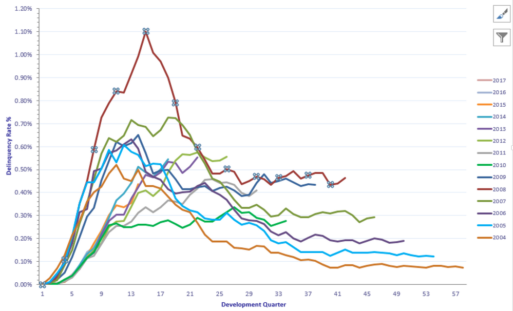
In this section we will adjust the original chart to remove all line styling and introduce mouse-over events on a single line level. The data used for this exercise is stored in more_data.csv.
Load the original line_chart_interactive.html file (without the changes applied in the first scenario) in your code editor. For a start, let’s remove the styling from the lines: instead of giving each line a unique id, let’s group all lines under a single class.
Locate the following snippet in your code:
lines.append("path")
    .attr("class", ids)
    .attr("d", function(d) { return line(d.values); });
Amend the class attribute as below:
lines.append("path")
    .attr("class", "line")
    .attr("d", function(d) { return line(d.values); });
Apply unified style to all lines by adding this to the styles.css file:
.line {
fill: none;
stroke: #d2d2d2;
}
All lines show in grey after the page reload:
Just as in the previous scenario, let’s create invisible hover areas to make the line selection more user-friendly. The new elements will be called ghost_lines in the code. Append the following bit to the end of LINES section.
const ghost_lines = lines.append("path")
    .attr("class", "ghost-line")
    .attr("d", function(d) { return line(d.values); });
The ghost lines are constructed the same way as the regular chart lines. The difference is set in the css file: their stroke is notably wider to increase the interactive area, and their opacity is set to 0:
.ghost-line {
fill: none;
stroke: #d2d2d2;
opacity: 0;
stroke-width: 10;
}
After the html file is reloaded the graph remains unchanged but a new element is added to each g group:
Mouse events will be added to the ghost lines. Go ahead and paste the following snippet to the EVENTS section:
svg.selectAll(".ghost-line")
    .on('mouseover', function() {
        const selection = d3.select(this).raise();
        selection
            .transition()
            .delay("100")
            .duration("10")
            .style("stroke","#ed3700")
            .style("opacity","1")
            .style("stroke-width","3");
    })
    .on('mouseout', function() {
    const selection = d3.select(this)
    selection
            .transition()
            .delay("100")
            .duration("10")
            .style("stroke","#d2d2d2")
            .style("opacity","0")
            .style("stroke-width","10");
    });
There are two events: a ghost line is made visible once the cursor moves over its area and disappears as the cursor leaves the line. The ghost line is made thicker and marked with red on a hover over. Note how the raise() method is used to bring the selected line forward.
This design technique focuses the viewer’s attention on a particular line. The chart legend can be adjusted to follow this idea: by making the following changes the series name representing the selected line will be automatically accentuated.
svg.selectAll(".ghost-line")
    .on('mouseover', function() {
        const selection = d3.select(this).raise();

        selection
            .transition()
            .delay("100").duration("10")
            .style("stroke","#ed3700")
            .style("opacity","1")
            .style("stroke-width","3");

        // add the legend action
        const legend = d3.select(this.parentNode)
                .select(".serie_label");

        legend
                .transition()
                .delay("100")
                .duration("10")
                .style("fill","#2b2929");
            })

    .on('mouseout', function() {
        const selection = d3.select(this)
        selection
            .transition()
            .delay("100")
            .duration("10")
            .style("stroke","#d2d2d2")
            .style("opacity","0")
            .style("stroke-width","10");

        // add the legend action
        const legend = d3.select(this.parentNode)
            .select(".serie_label");
        legend
            .transition()
            .delay("100")
            .duration("10")
            .style("fill","#d2d2d2");
    });
As the events were configured on a ghost line level, we need to go up to the group g to be able to select the series name. This is achieved using a d3 selection: d3.select(this.parentNode). The labels can be given a less vivid shade of grey to make the selected series stand out stronger. Amend the serie_label class in the css file to the following:
.serie_label {
fill: #d2d2d2;
font-family: Georgia;
font-size: 80%;
}
Reload the html file: now the chart label reacts to line selection too!
The selected line stands out from the chart allowing the viewer for its immediate recognition, trend analysis, and a visual comparison with the rest of the group.
For an alternative technique of line selection check out a very cool interactive multi-line chart based on a huge data set from Bureau of Labor Statistics (authored by Mike Bostock).
Follow me on Twitter for more data-sciency / data visualisation projects!
Code Samples
Scenario 1
line_chart_interactive.html:
<!DOCTYPE html>
<head>
<meta charset="utf-8">
<title>Multi Line Chart</title>
<script type="text/javascript" src="https://d3js.org/d3.v5.min.js"></script>
<link rel="stylesheet" type="text/css" href="styles.css">
<style></style>
</head>
<body>
<div id="container" class="svg-container"></div>
<script>
//------------------------1. PREPARATION------------------------//
//-----------------------------SVG------------------------------//
const width = 960;
const height = 500;
const margin = 5;
const padding = 5;
const adj = 30;
// we are appending SVG first
const svg = d3.select("div#container").append("svg")
    .attr("preserveAspectRatio", "xMinYMin meet")
    .attr("viewBox", "-"
          + adj + " -"
          + adj + " "
          + (width + adj *3) + " "
          + (height + adj*3))
    .style("padding", padding)
    .style("margin", margin)
    .classed("svg-content", true);

//-----------------------------DATA-----------------------------//
const timeConv = d3.timeParse("%d-%b-%Y");
const dataset = d3.csv("data.csv");
dataset.then(function(data) {
    var slices = data.columns.slice(1).map(function(id) {
        return {
            id: id,
            values: data.map(function(d){
                return {
                    date: timeConv(d.date),
                    measurement: +d[id]
                };
            })
        };
    });

//----------------------------SCALES----------------------------//
const xScale = d3.scaleTime().range([0,width]);
const yScale = d3.scaleLinear().rangeRound([height, 0]);
xScale.domain(d3.extent(data, function(d){
    return timeConv(d.date)}));

yScale.domain([(0), d3.max(slices, function(c) {
    return d3.max(c.values, function(d) {
        return d.measurement + 4; });
        })
    ]);

//-----------------------------AXES-----------------------------//
const yaxis = d3.axisLeft()
    .ticks((slices[0].values).length)
    .scale(yScale);

const xaxis = d3.axisBottom()
    .ticks(d3.timeDay.every(1))
    .tickFormat(d3.timeFormat('%b %d'))
    .scale(xScale);

//----------------------------LINES-----------------------------//
const line = d3.line()
    .x(function(d) { return xScale(d.date); })
    .y(function(d) { return yScale(d.measurement); });

let id = 0;
const ids = function () {
    return "line-"+id++;
}

//---------------------------TOOLTIP----------------------------//
const tooltip = d3.select("body").append("div")
    .attr("class", "tooltip")
    .style("opacity", 0)
    .style("position", "absolute");

//-------------------------2. DRAWING---------------------------//
//-----------------------------AXES-----------------------------//
svg.append("g")
    .attr("class", "axis")
    .attr("transform", "translate(0," + height + ")")
    .call(xaxis);

svg.append("g")
    .attr("class", "axis")
    .call(yaxis)
    .append("text")
    .attr("transform", "rotate(-90)")
    .attr("dy", ".75em")
    .attr("y", 6)
    .style("text-anchor", "end")
    .text("Frequency");

//----------------------------LINES-----------------------------//
const lines = svg.selectAll("lines")
    .data(slices)
    .enter()
    .append("g");

lines.append("path")
    .attr("class", ids)
    .attr("d", function(d) { return line(d.values); });

lines.append("text")
    .attr("class","serie_label")
    .datum(function(d) {
        return {
            id: d.id,
            value: d.values[d.values.length - 1]}; })
    .attr("transform", function(d) {
            return "translate(" + (xScale(d.value.date) + 10)
            + "," + (yScale(d.value.measurement) + 5 )+ ")"; })
    .attr("x", 5)
    .text(function(d) { return ("Serie ") + d.id; });

//---------------------------POINTS-----------------------------//
lines.selectAll("points")
    .data(function(d) {return d.values})
    .enter()
    .append("circle")
    .attr("cx", function(d) { return xScale(d.date); })
    .attr("cy", function(d) { return yScale(d.measurement); })
    .attr("r", 1)
    .attr("class","point")
    .style("opacity", 1);

//---------------------------EVENTS-----------------------------//
lines.selectAll("circles")
    .data(function(d) { return(d.values); } )
    .enter()
    .append("circle")
    .attr("cx", function(d) { return xScale(d.date); })
    .attr("cy", function(d) { return yScale(d.measurement); })
    .attr('r', 10)
    .style("opacity", 0)
    .on('mouseover', function(d) {
        tooltip.transition()
            .delay(30)
            .duration(200)
            .style("opacity", 1);

        tooltip.html(d.measurement)
            .style("left", (d3.event.pageX + 25) + "px")
            .style("top", (d3.event.pageY) + "px");

        const selection = d3.select(this).raise();

        selection
            .transition()
            .delay("20")
            .duration("200")
            .attr("r", 6)
            .style("opacity", 1)
            .style("fill","#ed3700");
    })
    .on("mouseout", function(d) {
        tooltip.transition()
            .duration(100)
            .style("opacity", 0);

        const selection = d3.select(this);

        selection
            .transition()
            .delay("20")
            .duration("200")
            .attr("r", 10)
            .style("opacity", 0);
    });

});
</script>
</body>
styles.css:
/* AXES */
/* ticks */
.axis line{
stroke: #706f6f;
stroke-width: 0.5;
shape-rendering: crispEdges;
}

/* axis contour */
.axis path {
stroke: #706f6f;
stroke-width: 0.7;
shape-rendering: crispEdges;
}

/* axis text */
.axis text {
fill: #2b2929;
font-family: Georgia;
font-size: 120%;
}

/* LINE CHART */
path.line-0 {
fill: none;
stroke: #ed3700;
}

path.line-1 {
fill: none;
stroke: #2b2929;
stroke-dasharray: 2;
}

path.line-2 {
fill: none;
stroke: #9c9c9c;
stroke-dasharray: 6;
}

.serie_label {
fill: #2b2929;
font-family: Georgia;
font-size: 80%;
}

/* TOOLTIP */
.tooltip {
fill: #2b2929;
font-family: Georgia;
font-size: 150%;
}

/* POINTS */
.point {
stroke: none;
fill: #9c9c9c;
data.csv:
text
date,A,B,C
20-Jul-2019,10,20,16
21-Jul-2019,11,22,18
22-Jul-2019,13,19,21
23-Jul-2019,11,17,22
24-Jul-2019,15,16,20
25-Jul-2019,16,19,18
26-Jul-2019,19,21,18
27-Jul-2019,22,25,15
28-Jul-2019,18,24,12
29-Jul-2019,14,20,16
30-Jul-2019,14,18,18
31-Jul-2019,16,18,21
01-Aug-2019,15,20,22
02-Aug-2019,14,21,19
Scenario 2
line_chart_interactive.html:
<!DOCTYPE html>
<head>
<meta charset="utf-8">
<title>Multi Line Chart</title>
<script type="text/javascript" src="https://d3js.org/d3.v5.min.js"></script>
<link rel="stylesheet" type="text/css" href="styles.css">
<style></style>
</head>
<body>
<div id="container" class="svg-container"></div>
<script>
//------------------------1. PREPARATION------------------------//
//-----------------------------SVG------------------------------//
const width = 960;
const height = 500;
const margin = 5;
const padding = 5;
const adj = 30;
// we are appending SVG first
const svg = d3.select("div#container").append("svg")
    .attr("preserveAspectRatio", "xMinYMin meet")
    .attr("viewBox", "-"
          + adj + " -"
          + adj + " "
          + (width + adj *3) + " "
          + (height + adj*3))
    .style("padding", padding)
    .style("margin", margin)
    .classed("svg-content", true);

//-----------------------------DATA-----------------------------//
const timeConv = d3.timeParse("%d-%b-%Y");
const dataset = d3.csv("more_data.csv");
dataset.then(function(data) {
    var slices = data.columns.slice(1).map(function(id) {
        return {
            id: id,
            values: data.map(function(d){
                return {
                    date: timeConv(d.date),
                    measurement: +d[id]
                };
            })
        };
    });

//----------------------------SCALES----------------------------//
const xScale = d3.scaleTime().range([0,width]);
const yScale = d3.scaleLinear().rangeRound([height, 0]);
xScale.domain(d3.extent(data, function(d){
    return timeConv(d.date)}));

yScale.domain([(0), d3.max(slices, function(c) {
    return d3.max(c.values, function(d) {
        return d.measurement + 4; });
        })
    ]);

//-----------------------------AXES-----------------------------//
const yaxis = d3.axisLeft()
    .ticks((slices[0].values).length)
    .scale(yScale);

const xaxis = d3.axisBottom()
    .ticks(d3.timeDay.every(1))
    .tickFormat(d3.timeFormat('%b %d'))
    .scale(xScale);

//----------------------------LINES-----------------------------//
const line = d3.line()
    .x(function(d) { return xScale(d.date); })
    .y(function(d) { return yScale(d.measurement); });

//-------------------------2. DRAWING---------------------------//
//-----------------------------AXES-----------------------------//
svg.append("g")
    .attr("class", "axis")
    .attr("transform", "translate(0," + height + ")")
    .call(xaxis);

svg.append("g")
    .attr("class", "axis")
    .call(yaxis)
    .append("text")
    .attr("transform", "rotate(-90)")
    .attr("dy", ".75em")
    .attr("y", 6)
    .style("text-anchor", "end")
    .text("Frequency");

//----------------------------LINES-----------------------------//
const lines = svg.selectAll("lines")
    .data(slices)
    .enter()
    .append("g");

    lines.append("path")
    .attr("class", "line")
    .attr("d", function(d) { return line(d.values); });

    lines.append("text")
    .attr("class","serie_label")
    .datum(function(d) {
        return {
            id: d.id,
            value: d.values[d.values.length - 1]}; })
    .attr("transform", function(d) {
            return "translate(" + (xScale(d.value.date) + 10)
            + "," + (yScale(d.value.measurement) + 5 )+ ")"; })
    .attr("x", 5)
    .text(function(d) { return ("Serie ") + d.id; });

const ghost_lines = lines.append("path")
    .attr("class", "ghost-line")
    .attr("d", function(d) { return line(d.values); });

//---------------------------EVENTS-----------------------------//
svg.selectAll(".ghost-line")
    .on('mouseover', function() {
        const selection = d3.select(this).raise();

        selection
            .transition()
            .delay("100").duration("10")
            .style("stroke","#ed3700")
            .style("opacity","1")
            .style("stroke-width","3");

        // add the legend action
        const legend = d3.select(this.parentNode)
            .select(".serie_label");

        legend
            .transition()
            .delay("100")
            .duration("10")
            .style("fill","#2b2929");
        })

    .on('mouseout', function() {
        const selection = d3.select(this)

        selection
            .transition()
            .delay("100")
            .duration("10")
            .style("stroke","#d2d2d2")
            .style("opacity","0")
            .style("stroke-width","10");

        // add the legend action
        const legend = d3.select(this.parentNode)
            .select(".serie_label");

        legend
            .transition()
            .delay("100")
            .duration("10")
            .style("fill","#d2d2d2");
    });
});
</script>
</body>
styles.css:
/* AXES */
/* ticks */
.axis line{
stroke: #706f6f;
stroke-width: 0.5;
shape-rendering: crispEdges;
}

/* axis contour */
.axis path {
stroke: #706f6f;
stroke-width: 0.7;
shape-rendering: crispEdges;
}

/* axis text */
.axis text {
fill: #2b2929;
font-family: Georgia;
font-size: 120%;
}

/* LINE CHART */
.line {
fill: none;
stroke: #d2d2d2;
}

.ghost-line {
fill: none;
stroke: #d2d2d2;
opacity: 0;
stroke-width: 10;
}

.serie_label {
fill: #d2d2d2;
font-family: Georgia;
font-size: 80%;
}
more_data.csv:
date,A,B,C,D,E,F,G,H,I,J
20-Jul-2019,10,20,16,8,19,18,12,9,10,15
21-Jul-2019,11,22,18,10,21,22,11,9,12,15
22-Jul-2019,13,19,21,11,22,20,8,10,12,17
23-Jul-2019,11,17,22,15,23,19,10,9,14,16
24-Jul-2019,15,16,20,12,24,22,11,13,15,16
25-Jul-2019,16,19,18,11,22,22,13,13,14,16
26-Jul-2019,19,21,18,10,25,23,14,14,16,14
27-Jul-2019,22,25,15,14,27,23,15,12,17,15
28-Jul-2019,18,24,12,14,25,20,14,10,18,16
29-Jul-2019,14,20,16,17,27,17,14,12,17,18
30-Jul-2019,14,18,18,14,28,17,14,8,19,17
31-Jul-2019,16,18,21,13,30,15,15,7,22,20
01-Aug-2019,15,20,22,12,28,16,13,7,20,19
02-Aug-2019,12,21,19,10,28,17,14,8,20,22